
The cryptocurrency market is so huge that it’s confusing to most of us. The global crypto market cap is $2.44T right now. The value of the currencies fluctuates every now and then. But there must be a way to predict its prices, right?
We will use time-series data for cryptocurrencies such as Bitcoin, Ethereum, and Ripple and predict crypto prices in this article. Given the market uncertainty surrounding various cryptocurrency prices, we decided to test a simple neural network on publicly accessible data (till 2018) to see whether we could predict crypto prices with fair accuracy without using any significant computational resources. CoinMarketCap provided the data for this test.
How to collect cryptocurrency data?
The total crypto market volume over the last 24 hours is $231.54 Billion, indicating an 8.28% decrease. Devi’s overall volume is reported at $18.43 billion now, 7.96 per cent of the total 24-hour volume in the crypto market. The overall value of all stable coins is now $180.71B, which reflects 78.05 per cent of the total 24-hour volume of the crypto market. (Till May 10, 2021)
The data for each currency is from the day it was introduced or when it began to generate any market value till 2018. For Bitcoin (BTC), the data ranges from April 28, 2013, to the fiscal year 2018. And, it is from August 7, 2015, for Ethereum (ETH).
Understand cryptocurrency terms
There are a total of six major features in the data. The following are the descriptions for them:
- Close Price – This is the currency’s market close price for that specific day;
- Open Price – This is the currency’s market open price for that particular day;
- High Price – It is the day’s highest currency price;
- Low Price – It is the day’s lowest currency price;
- Volume – The volume of currency traded on that particular day.
- Market Cap – The overall market capitalization of a currency on that particular day. It can differ tremendously on any given day, depending on market fluctuations.
Correlation Between The Cryptocurrencies
To begin with, let us analyze the relationship between some of these cryptocurrencies.
According to Cryptowatch, the correlation between the cryptos is described as, “Positively correlated variables tend to move together, negatively correlated variables move inversely to each other, and uncorrelated variables move independently of each other.”
Here’s what the chart looks like for the last 7 days.
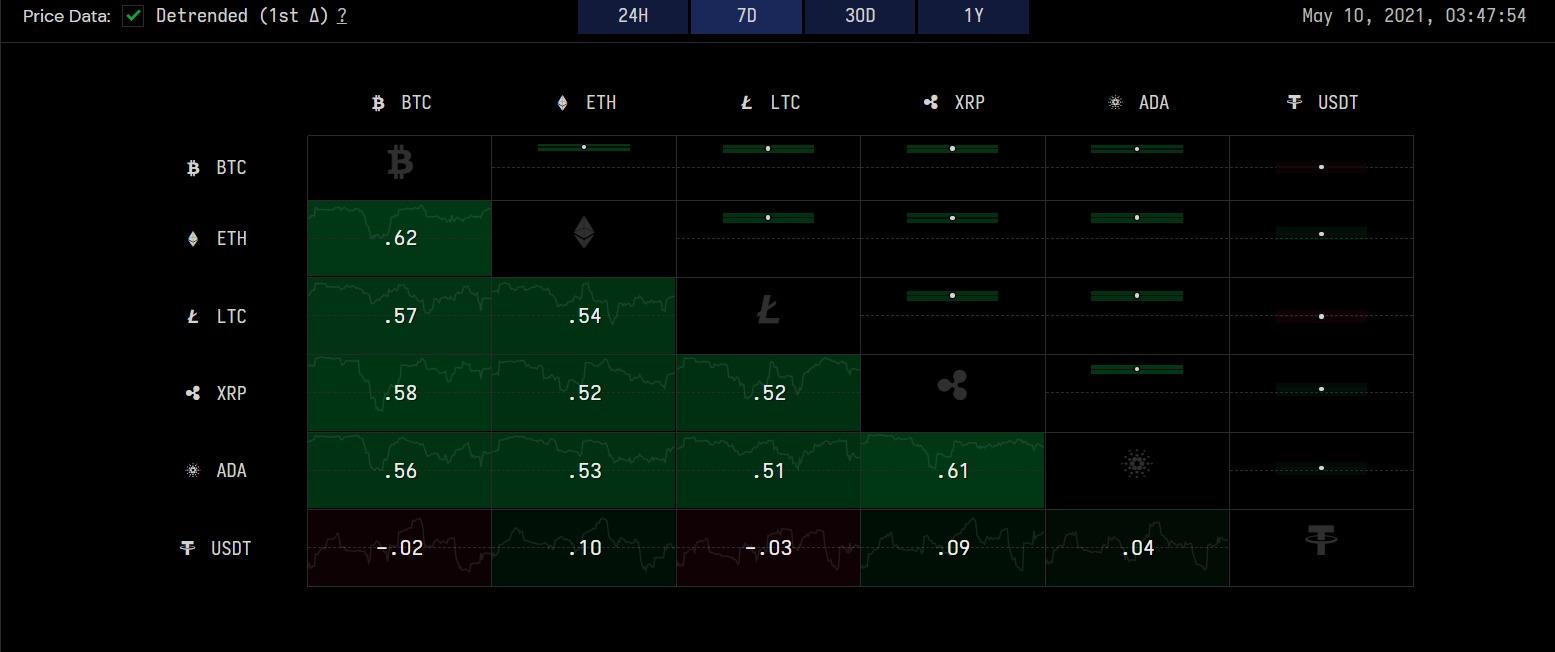
Here the green ones indicate a positive value, i.e., a positive correlation between two variables, whereas the red ones indicate a negative correlation or a negative value.
These values are called the Pearson Correlation Coefficient. It quantifies the estimated strength of the linear association between two variables. And it ranges from +1 to -1. However, it’s unlikely to get a coefficient of +1 which means a perfect linear correlation. Besides, -1 indicates a negative linear correlation. This chart indicates the change in correlation between the cryptocurrencies over time.
Now, by using the data collected from CoinMarketCap, let’s see if we can predict the prices of the cryptos.
Using The LSTM Neural Network To Predict “Close Prices”
Overall, to predict “close prices” using an LSTM neural network, we followed the following steps.
- Using Keras, build an LSTM model
- Normalize data by MinMaxScaler from Scikit-Learn
- Re-frame data for supervised learning using Pandas
- Train the LSTM model on a training data set
- Close price testing/prediction
Given that we’re dealing with time series analysis, LSTM is an excellent choice. Long short-term memory (LSTM) units (or blocks) are the foundations for layers of Recurrent Neural Network (RNN). An LSTM network is an RNN comprised of LSTM units.
The word “long short-term memory” alludes to the fact that LSTM is a model for short-term memory that can last for a long time. An LSTM is well-suited to characterize, process, and forecast time series with uncertain time lags between major events. When training traditional RNNs, LSTMs were designed to deal with the exploding and vanishing gradient problem. In many applications, LSTM’s relative insensitivity to gap length gives it an advantage over alternative RNNs, hidden Markov models, and other sequence learning methods.
Felix A. GersDouglas, EckJürgen, and Schmidhuber’s 2001 paper Applying LSTM to Time Series Predictable through Time-Window Approaches demonstrate the promising effects of LSTM on time series data. The authors of the paper demonstrated LSTM solving two difficult time-series challenges. Firstly, they tried to solve the Mackey-Glass Series. Secondly, they addressed another problem, the Chaotic Laser Data (Set A). Both data sets are considered benchmarks for time-series analysis. For more details, click here! In our model, we are creating a simple LSTM in Keras. Keras is a deep learning framework and high-level API wrapper that runs on top of Tensorflow or Caffe2. It also makes use of GPU capabilities. As a result, it is an excellent alternative for basic models.
Building the cryptocurrency model
Our model architecture is straightforward. It has 75 to 80 neurons in its network. The Adam optimizer is being used here to optimize the loss function, which will be the Mean Absolute Error (MAE). Commonly people use RMSE (Root Mean Square Error), but we will stick with the traditional method.
The code snippet below shows how to build an LSTM model with Keras.
# design network
model = Sequential()
model.add(LSTM(80, input_shape=(train_X.shape[1], train_X.shape[2])))
model.add(Dense(1))
model.compile(loss='mae', optimizer='adam')
history = model.fit(train_X, train_y, epochs=50, batch_size=32, validation_data = (tesst_X, test_y), verbose=2, shuffle=False)

# plot history
pyplot.plot(history,history['loss'], label = 'train')
pyplot.ploy(history.history['val_loss'], label = 'test')
pyplot.legend()
pyplot.show()
Now that we have data and a model, let’s dive right in for the next steps.
Normalizing the price data
We have data with different values ranging from 10,000 USD to 216740000000 USD for Market Cap. This is not a suitable model to understand. So, we’ll use Scikit-Learn to normalize our data by using MinMaxScaler.
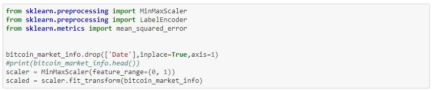
The code above normalizes the Bitcoin data to a zero mean and a standard deviation of one.
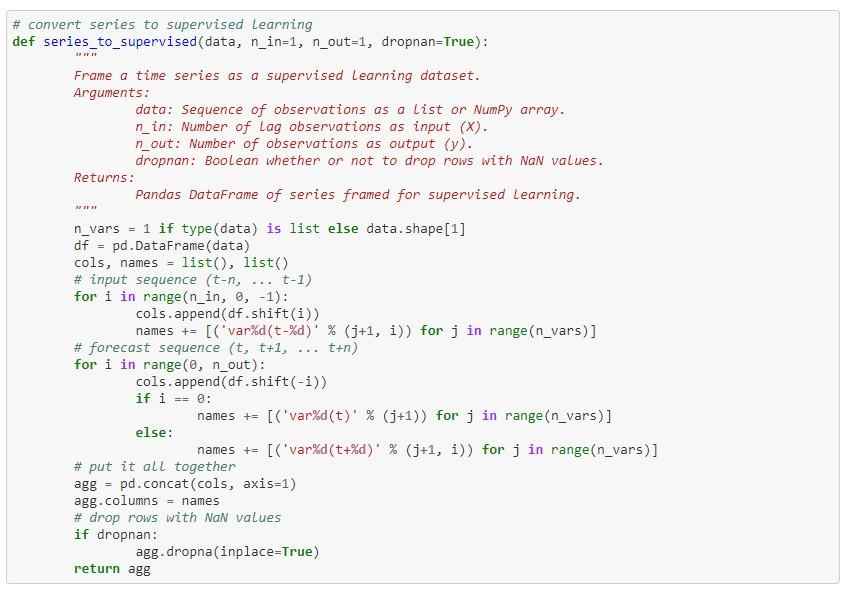
Re-framing Data For Supervised Learning
Since the data is time-series, we must prepare it in such a way that we can forecast the next day’s close price as output for the current day’s data. We are using the function shown below to create the data.
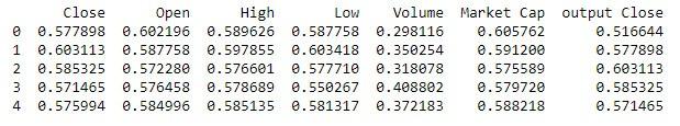
When we apply the above function to our Bitcoin data, we get newly re-framed data, and the first five outputs of the re-framed data are shown below in the normalized form.
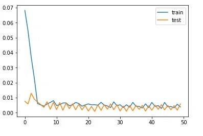
Training The LSTM Model
We now have our model, as well as the prepared data. It’s time to train the model to see how well it does on the testing dataset. We will train the LSTM model for 50 epochs (number of training iterations) in a batch size of 32. The loss would then be plotted against epochs for both the train and test sets. The Bitcoin plot looks like this:
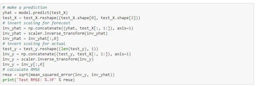
We will use the following code to test our model:
Predict cryptocurrency prices results
We used the data publicly accessible till 2018 and predicted the following results.
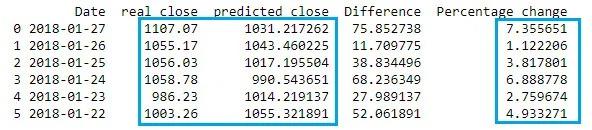
Bitcoin price prediction
According to our tests, Bitcoin close prices from 22 to 27 January 2018, and comparing them to actual close prices on those days, the chart looks like this.

According to the data presented above, our prediction model worked fairly well, with expected close prices and actual close prices differing by 0 to 5.1 percent. The largest difference is approximately $586, with a percentage difference of approximately 5.1 percent as compared to the actual close price.
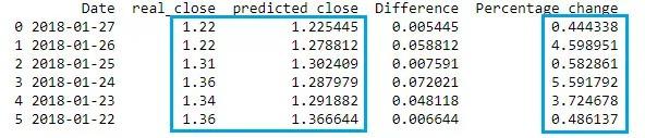
Ethereum price prediction
We also predicted for Ethereum from 21 January to 27 January 2018 to see how this test performs on unseen data. So this is what we get for Ethereum in the table below.
As seen above, the difference between the actual and expected close prices ranges from 0% to 7.4%.
Ripple price prediction
On Ripple data, we trained the same LSTM model. The results are shown in the table below.
Again, the overall difference between actual and expected prices ranges between 0 and 5.6 percent.
There’s another such tool called Fibonacci retracement. Let’s find out what it is and how it works.
Fibonacci Retracement Price Prediction
Fibonacci retracement is used to detect potential trend reversals, such as when a growing market will decline or a declining market will rise. As a result, it indicates the potential entry point in a trade. You can sell if you can predict the price will fall with a level of certainty. You can buy if you can predict with an assurance that the price will grow.
The Fibonacci sequence is the foundation of Fibonacci retracement. Except for the first two numbers, 0 and 1, the Fibonacci sequence is a set of numbers obtained from adding the previous two numbers in the series.
The sequence is: 0, 1, 1, 2, 3, 5, 8, 13, 21, 34, 55, 89, 144, 233, 377, 610……
The prediction Process
Calculation 1
Divide each number in the series by the number that is two places higher in the sequence than itself. For instance, divide 2 by 5, 5 by 13, and divide 13 by 34, and so on. You get the gist of it. Even if you’re not Sherlock Holmes, you can tell that all of the answers are really close to .382. So, just keep the number.382 in mind.
Calculation 2
Divide each number in the series by the number that follows it in the sequence. For example, divide 5 by 8, 8 by 13, 55 by 89, and so on. You’re getting closer to another magical number,.618.
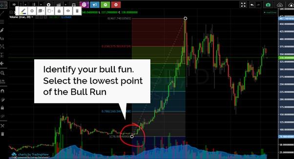
The Fibonacci retracement is used on a bullish or bearish run. When applying on a bullish run, you choose the lowest point or the potential start of the run. Take a look at the graph below.
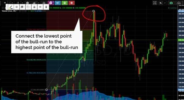
Likewise, select the highest point where the bullish run stopped. Such as:
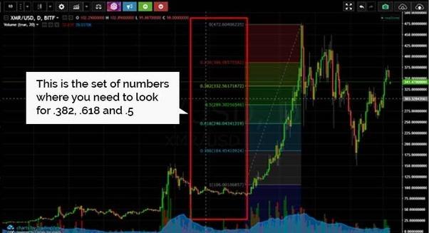
When you use a Fibonacci retracement on a candlestick graph, you will notice a sequence of numbers on the y-axis.
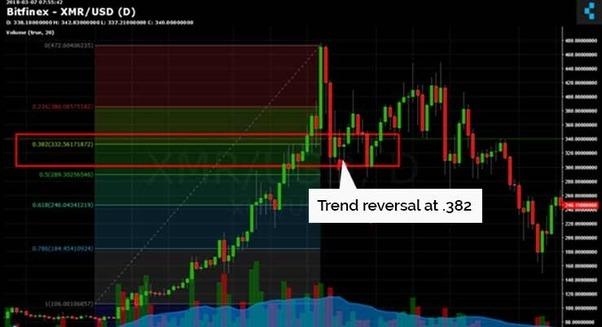
As you can see, the price was falling until it reached 0.382 level and then reversed.
According to experts, the best point of entry into a trade is between 0.618 and 0.786; this is the ideal trade entry point.
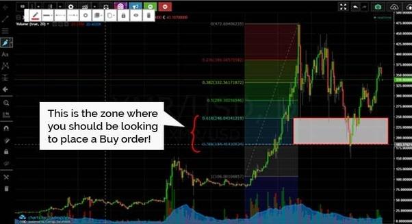
Similar trends apply to bear markets too.
You need to keep in mind that none of these methods/tools will give the right results every time. You need to be always updated.
Final Words
We showed how deep learning could be used to predict cryptocurrency prices using time series data. We used a simple LSTM network. Bidirectional LSTM networks can also be used; the training model can be run for a longer period of time and fine-tuned for greater precision. To predict outcomes, a similar approach can be used with other financial time series data.
The source code repository is available here if you want to try out the LSTM model Pirimid Fintech developed.
We also showed how we could use Fibonacci Retracement to predict the best entry point. All these will work as long as you are well informed about the currencies. No method is fool-proof. But with the help of this article, you should be able to predict the prices of cryptocurrencies with a fair level of accuracy.